Quantifying the Transferability of Sim-to-Real Control Policies

2019, Feb 21    

This post is about how we can quantitatively estimate the transferability of a control policy learned from randomized simulations pertaining to physical parameters of the environment. Learning continuous control policies in the real world is expensive in terms of time (e.g., gathering the data) and resources (e.g., wear and tear on the robot). Therefore, simulation-based policy search appears to be an appealing alternative.

Learning from Physics Simulations

In general, learning from physics simulations introduces two major challenges:

1. Physics engines (e.g., Bullet, MoJoCo, or Vortex) are build on models, which are always an approximation of the real world and thus inherently inaccurate. For the same reason, there will always be unmodeled effects.

2. Sample-based optimization (e.g., reinforcement learning) is known to be optimistically biased. This means, that the optimizer will over-fit to the provided samples, i.e., optimize for the simulation and not for the real problem, which the one we actually want to solve.

The first approach to make control policies transferable from simulation to the reality, also called bridging the reality gap, was presented by Jakobi et al.. The authors showed that by adding noise to the sensors and actors while training in simulation, it is possible to yield a transferable controller. This approach has two limitations: first, the researcher has to carefully select the correct magnitude of noise for every sensor and actor, second the underlying dynamics of the system remain unchanged.

Domain Randomization

One possibility to tackle the challenges mentioned in the previous section is by randomizing the simulations. The most prominent recent success using domain randomization is the robotic in-hand manipulation of physical objects, described in a blog post from OpenAI.

A domain is one instance of the simulator, i.e., a set of domain parameters describes the current world our robot is living in. Basically, domain parameters are the quantities that we use to parametrize the simulation. This can be physics parameters like the mass and extents of an object, as well as a gearbox’s efficiency, or visual features like textures camera positions.

Loosely speaking, randomizing the physics parameters can be interpreted as another way of injecting noise into the simulation while learning. In contrast to simply adding noise to the sensors and actors, this approach allows to selectively express the uncertainty on one phenomenon (e.g., rolling friction). The motivation of domain randomization in the context of learning from simulations is the idea that if the learner has seen many variations of the domain, then the resulting policy will be more robust towards modeling uncertainties and errors. Furthermore, if the learned policy is able to maintain its performance across an ensemble of domains, it is more like to transferable to the real world.

What to Randomize

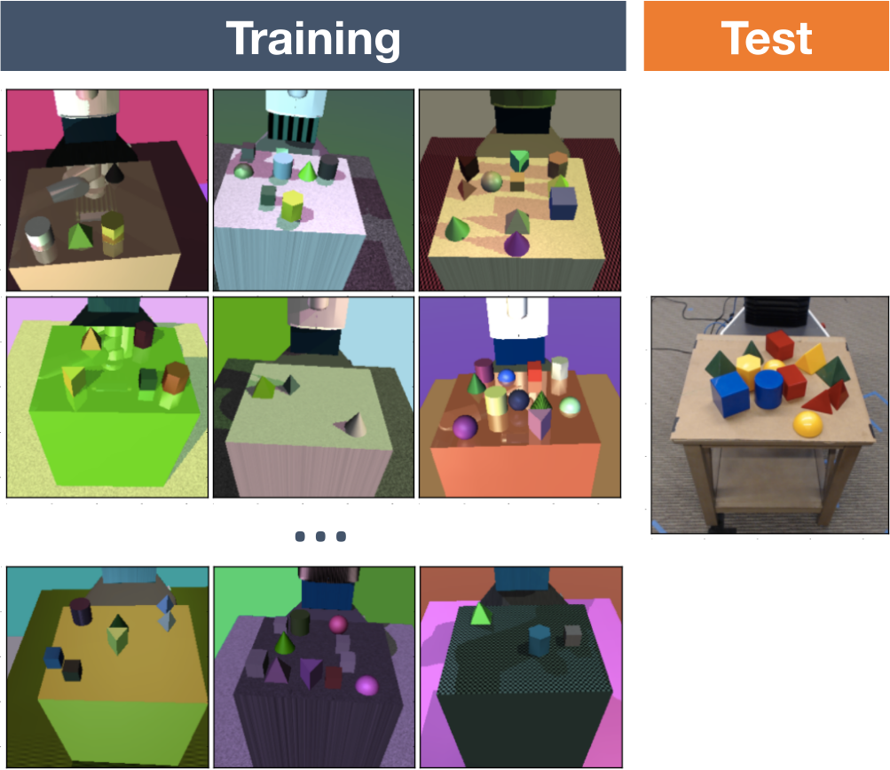
A lot of research in the sim-to-real field has been focused on randomizing visual features (e.g., textures, camera properties, or lighting). Examples are the work of Tobin et al., who trained an object detector for robot grasping (see figure to the right), or the research done by Sadeghi and Levine, where a drone learned to fly from experience gathered in visually randomized environments.

In this blog post, we focus on the randomization of physics parameters (e.g., masses, centers of mass, friction coefficients, or actuator delays), which change the dynamics of the system at hand. Depending on the simulation environment, the influence of some parameters can be crucial, while other can be neglected.

To illustrate this point, we consider a ball rolling downhill on a inclined plane. In this scenario, the ball’s mass as well as radius do not influence how fast the ball is rolling. So, varying this parameters while learning would be a waste of computation time. Note: the ball’s inertia tensor (e.g., solid or hollow sphere) does have an influence.

How to Randomize

After deciding on which domain parameters we want to randomize, we must decide how to do this. Possible approaches are:

1. Sampling domain parameters from static probability distributions
   This approach is the most widely used of the listed. The common element between the different algorithms is that every domain parameter is randomized according to a specified distribution. For example, the mechanical parts of a robot or the objects it should interact with have manufacturing tolerances, which can be used as a basis for designing the distributions. This sampling method is advantageous since it does not need any real-world samples, and the hyper-parameters (i.e., the parameters of the probability distributions) are easy to interpret. On the downside, the state-of-the-art hyper-parameter selection done by the researcher and can be potentially time-intensive. Examples of this randomization strategy are for example the work by OpenAI, Rajeswaran et al., and Muratore et al.

2. Sampling domain parameters from adaptive probability distributions
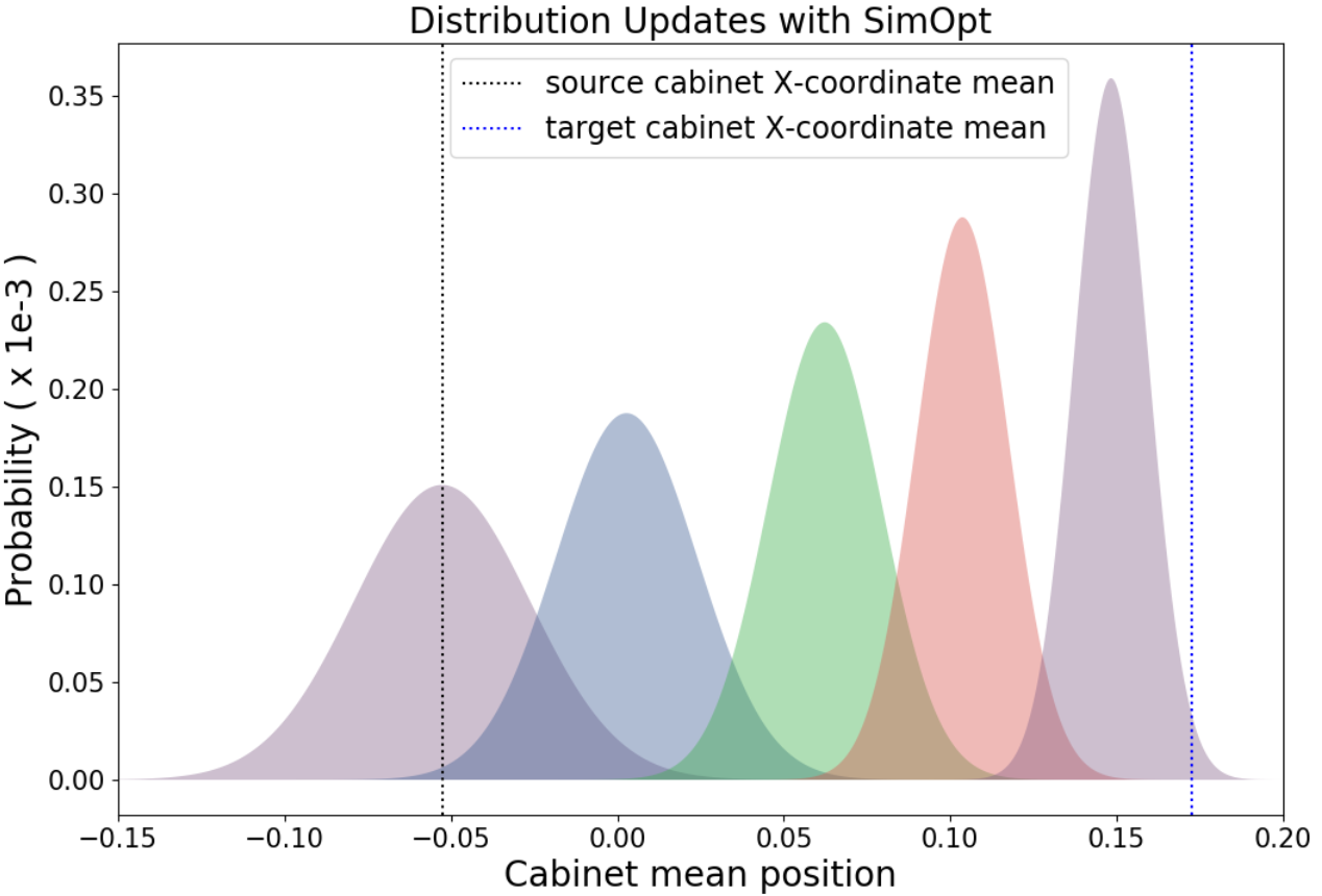   Chebotar et al. presented a very promising method on how to close the sim-to-real loop by adapting the distributions from which the domain parameters are sampled depending on results from real-world rollouts (see figure to the right). The main advantage is, that this approach alleviates the need for hand-tuning the distributions of the domain parameters, which is currently a significant part of the hyper-parameter search. On the other side, the adaptation requires data from the real robot which expensive. For this reason, we will only focus on methods that sample from static probability distributions.

3. Applying adversarial perturbations
   One could argue that technically these approaches do not fit the domain randomization category, since the perturbations are not necessarily random. Nonetheless, we think this concept is an interesting compliment to the previously mentioned sampling methods. In particular, we want to highlight the following two ideas. Mandlekar et al. proposed physically plausible perturbations of the domain parameters by randomly deciding (Bernoulli experiment) when to add a rescaled gradient of the expected return w.r.t. the domain parameters. Moreover,the paper includes an ablation analysis on the effect of adding noise to the domain parameters or directly to the states. Pinto et al. suggested to add a antagonist agent whose goal is to hinder the protagonist agent (the policy to be trained) from fulfilling its task. Both agents are trained simultaneously and make up a zero-sum game.
   In general, adversarial approaches may provide a particularly robust policy. However, without any further restrictions, it is always possible create scenarios in which the protagonist agent can never win, i.e., the policy will not learn the task.

Interestingly, most recent work is focussed on randomising the domain parameters in a per-episode fashion, i.e., once at the beginning of every rollout (excluding the adversarial approaches mentioned in the list above). Alternatively, one could randomize the parameters every time step. We believe there could be few reasons to randomize once per rollout. First, it is harder to implement from the physics engine point of view. Second, the very frequent parameter changes are most likely detrimental to learning, because the resulting dynamics would become significantly nosier.

Quantifying the Transferability During Learning

In the state-of-the-art of sim-to-real reinforcement learning, there are several algorithms which learn (robust) continuous control policies in simulation. Some of them already showed the ability to transfer from simulation to reality. However, all of these algorithms lack a measure of the policy’s transferability and thus they just train for a given number of rollouts or transitions. Usually, this problem is bypassed by training for a “very long time” (i.e., using a “huge amount” of samples) and then testing the resulting policy on the real system. If the performance is not satisfactory, the procedure is repeated.

Muratore et al. presented an algorithm called Simulation-based Policy Optimization with Transferability Assessment (SPOTA) which is able to directly transfer from an ensemble of source domains to an unseen target domain. The goal of SPOTA is not only to maximize the agent’s expected discounted return under the influence of perturbed physics simulations, but also to provide an approximate probabilistic guarantee on the loss in terms of this performance mueasure when applying the found policy $\pi(\theta)$, a mapping from states to actions, to a different domain.

We start by framing reinforcement learning problem as a stochastic program, i.e., maximizing the expectation of estimated discounted return $J(\theta)$ over the domain parameters $\xi \sim p(\xi; \psi)$, where $\psi$ are the parameters of the distribution

$$J(\theta^{\star}) = \max_{\theta \in \Theta} \mathbb{E}_\xi \left[J(\theta, \xi) \right].$$

Since it is intractable to compute the expectation over all domains, we approximate the stochastic program using $n$ samples

$$\hat{J}_n(\theta^{\star}_n) = \max_{\theta \in \Theta} \frac{1}{n}\sum_{i=1}^{n} J(\theta, \xi_i).$$

It has been shown under mild assumptions, which are fulfilled in the reinforcement leaning setting, that sample-based optimization is optimistically biased, i.e., the solution is guaranteed to degrade in terms of performance when transformed to the real system. This loss in performance can be expressed by the Simulation Optimization Bias (SOB)

$$\mathrm{b}\left[ \hat{J}_n(\theta^{\star}_n) \right] = \underbrace{ \mathbb{E}_\xi \left[ \max_{\hat{\theta} \in \Theta} \frac{1}{n}\sum_{i=1}^{n} J(\hat{\theta}, \xi_i) \right] }_{\text{optimal value for samples}} - \underbrace{ \max_{\theta \in \Theta} \mathbb{E}_\xi \left[ J(\theta, \xi) \right] }_{\text{true optimal value}} \ge 0.$$

The figure below qualitatively displays the SOB between the true optimum $J(\theta^\star)$ and the sample-based optimum $\hat{J}_n(\theta_n^\star)$. The shaded region visualizes the variance arising when approximating $J(\theta)$ with $n$ domains.

Unfortunately, this quantity can not be used right away as an objective function, because we can not compute the expectation in the minuend, and we do not know the optimal policy parameters for the real system $\theta^\star$ in the subtrahend. Inspired by the work of Mak et al. on assessing the solution quality of convex stochastic problems, we employ the Optimality Gap (OG) at the candidate solution $\theta^c$

$$G(\theta^c) = \underbrace{\max_{\theta \in \Theta} \mathbb{E}_\xi \left[J(\theta, \xi) \right]}_{\text{best solution's value}} - \underbrace{\mathbb{E}_\xi \left[J(\theta^c, \xi) \right]}_{\text{candidate solution's value}} \ge 0$$

to quantify how much our solution $\theta^c$, e.g. yielded by a policy search algorithm, is worse than the best solution the algorithm could have found. In general, this measure is agnostic to the fact if we are evaluating the policies in simulation or reality. Since we are discussing the sim-to-real setting, think of OG as a quantification of our solutions suboptimality in simulation. However, computing $G(\theta^c)$ also includes an expectation over all domains. Thus, we have to approximate it from samples. Using $n$ domains, the estimated OG at our candidate solution is

$$\hat{G}_n(\theta^c) = \max_{\theta\in\Theta} \hat{J}_n(\theta) - \hat{J}_n(\theta^c) \ge G(\theta^c).$$

In SPOTA, an upper confidence bound on $\hat{G}_n(\theta^c)$ is used to give a probabilistic guarantee on the transferability of the policy learned in simulation. So, the results is a policy that with probability $(1-\alpha)$ does not lose more than $\beta$ in terms of return when transferred from one domain to a different domain of the same source distribution $p(\xi; \psi)$. Essentially, SPOTA increases the number of domains for every iteration until the policy’s upper confidence bound on the estimated OG is lower than the desired threshold $\beta$.

Let’s assume everything worked out fine and we trained a policy from randomized simulations such that the upper confidence bound on $\hat{G}_n(\theta^c)$ was reduced below the desired threshold. Now, the key question is if this property actually contributes to our goal of obtaining a low Simulation Optimization Bias (SOB). The relation between the OG and and the SOB can be written as

$$\mathrm{b}\left[ \hat{J}_n(\theta^{\star}_n) \right] = \mathbb{E}_\xi \left[ \hat{G}_n(\theta^c) \right]- G(\theta^c)$$

where in this case the evaluation is performed in the real world. Therefore, lowering the upper confidence bound on the estimated OG $\hat{G}_n(\theta^c)$ contributes to lowering the SOB $\mathrm{b}\left[ \hat{J}_n(\theta^{\star}_n) \right]$.

Please note, that the terminology used in this post deviates sightly from the one used in Muratore et al..

SPOTA — Sim-to-Sim Results

Preceding results on transferring policies trained with SPOTA from one simulation to another have been reported in Muratore et al.. The videos below show the performance in example scenarios side-by-side with 3 baselines:

• EPOpt by Rajeswaran et al. which is a domain ranomization algorithm that maximizes the conditional value at risk of the expected discounted return
• TRPO without domain randomization (implementation from Duan et al.)
• LQR applying optimal control for the system linearized around the goal state (an equilibrium)

SPOTA — Sim-to-Real Results

Finally, we want to share some early results acquired on the 2 DoF Ball Balancer from Quanser. Here, the task is to stabilize a ball at the center of the plate. The device receives voltage commands for the two motors and yields measurements of the ball position (2D relative to the plate) as well as the motors’ shaft angular positions (relative to their initial position). Including the velocities derived from the position signals, the system has a 2-dim continuous action space and a 8-dim continuous observation space.

Assume we obtained an analytical model of the dynamics and determined the parameters with some imperfections (e.g., the characteristics of the servo motors from the data sheet do not match the reality).

In the first experiment, we investigate what happens if we train control policies on a slightly faulty simulator using a model-free reinforcement learning algorithm called Proximal Policy Optimization (PPO).

Left video: a policy learned with PPO on a simulator with larger ball and larger plate— tested on the nominal system.
Right video: another policy learned with PPO on a simulator with higher motor as well as gear box efficiency— tested on the nominal system.

In the second experiment, we test policies trained using SPOTA, i.e., applying domain randomization.

Left video: a policy learned with SPOTA— tested on the nominal system.
Right video: the same policy learned with SPOTA— tested with a modified ball (the ball was cut open and filled with paper, the remaining glue makes the ball roll unevenly).

Disclaimer: despite a dead band in the servo motors’ voltage commands, noisy velocity signals from the ball detection, and (minor) nonlinearities in the dynamics this stabilizing task can also be solved by tuning the gains of a PD-controller while executing real-world trials. Furthermore, after a careful parameter estimation, we are able to learn this task for the nominal system in simulation using PPO. However, the resulting policy is sensitive to model uncertainties (e.g., testing with a different ball).

Author

Fabio Muratore — Intelligent Autonomous Systems Group (TU Darmstadt) and Honda Research Institute Europe

Acknowledgements

We would like to thank Ankur Handa for editing and Michael Gienger for proofreading this post.

Credits

First figure with permission from Josh Tobin (source)
Second figure with permission from Yevgen Chebotar (source)