Understanding Physics Engines: Dynamic Models of Manipulators

2020, Mar 01    

Physics engines simulate a carefully approximated and idealised version of the real world. In recent times, the popularity of physics simulators has only increased among machine learning and computer vision practicioners. Being able to forward simulate the evolution of a physical world as a function of time — under certain set of assumptions and approximations — allows for optimising a control policy to carry out tasks. In this post, we will dive into the underlying maths and derive the fundamental equation that all physics engines implement to simulate dynamic model of an articulated manipulator, i.e. how does the applied torque relate to the joint velocity and acceleration given joint properties like mass, friction and gravity. It is formulated as:

$$M(q)\ddot q + C(q, \dot q) \dot q + g(q) = \tau$$

where

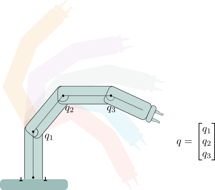
• $q$ is the vector of generalized coordinates, for instance the vector of joint-angles for a manipulator,
• $\dot q$ is the velocity of $q$,
• $\ddot q$ is the acceleration of $q$,
• $M(q)$ is the $n \times n$ generalised inertia matrix,
• $C(q, \dot q)$ is $n \times n$ matrix and $C(q, \dot q) \dot q$ is $n \times 1$ vector of centripetal and coriolis terms,
• $g(q)$ is $n \times 1$ vector of gravity terms, and
• $\tau$ is $n \times 1$ vector of joint torques.

This equation provides the relation between the applied forces/torques and the resulting motion of a manipulator. Similar to kinematics, it is also possible to define two dynamics “models”:

Forward model: once the forces/torques applied to the joints, as well as the joint positions and velocities are known, compute the joint accelerations:

$$\ddot q = M(q)^{-1}\bigg(\tau - C(q, \dot q) \dot q - g(q)\bigg)$$

and then

$$\dot q = \int \ddot q dt , \hspace{10mm} q = \int \dot q dt$$

Inverse model: once the joint accelerations, velocities and positions are known, compute the corresponding forces/torques

$$\tau = M(q)\ddot q + C(q, \dot q) \dot q + g(q)$$

This equation can be derived using either Newton-Euler method or the Lagrangian mechanics via Euler-Lagrange which is what we do here in this post. The Largrangian mechanics deals with energies of the system and from physics we know that it is possible to define:

• The kinetic energy of the system, $\mathcal{K}(q, \dot q)$
• Potential energy of the system, $\mathcal{P}(q)$

The Lagrangian is $\mathcal{L}(q, \dot q) = \mathcal{K}(q, \dot q) - \mathcal{P}(q)$.

One may think of a physical system, changing as time goes on from one state or configuration to another, as progressing along a particular evolutionary path, and ask, from this point of view, why it selects that particular path out of all the paths imaginable. The answer is that the physical system sums the values of its Lagrangian function for all the points along each imaginable path and then selects that path with the smallest result. The Lagrangian function measures something analogous to increments of distance, in which case one may say, in an abstract way, that physical systems always take the shortest paths. Source: https://www.britannica.com/science/Lagrangian-function

The Euler-Lagrange equations are defined as

$$\psi_i = \frac{d}{dt} \bigg( \frac{\partial \mathcal{L}}{\partial \dot q_i} \bigg) - \frac{\partial \mathcal{L}}{\partial q_i} \hspace{10mm} i = 1, 2, \cdots, n$$

Let us denote the $i^{th}$ joint by $q_i$ with $\psi_i$ being the non-conservative (external or dissipative) generalised forces performing any work on the joints $q_i$. It can be decomposed into:

• $\tau_i$, the joint actuator torque.
• $J_i^\top F_{c_i}$, the term due to external forces.
• $d_{ii} \dot q_i$, joint friction torque.

Therefore, it can be written as $\psi_i = \tau_i + J_i^\top F_{c_i} - d_{ii}\dot q_i$. Since the potential energy does not depend on the velocity, the euler-lagrange equation can be further simplied as

$$\psi_i = \frac{d}{dt} \bigg( \frac{\partial \mathcal{K}}{\partial \dot q_i} \bigg) - \frac{\partial \mathcal{K}}{\partial q_i} + \frac{\partial \mathcal{P}}{\partial q_i}$$

Where $\mathcal{K} = \sum_{i=1}^{n}\mathcal{K}_i \hspace{10mm} \mathcal{P} = \sum_{i=1}^{n}\mathcal{P}_i$.

Computing Kinetic Energy

For any rigid body B, the mass can be computed by integrating the mass density as:

$$m = \int_{B} \rho(x, y, z)\hspace{1mm} dx dy dz$$

where the term $\rho(x, y, z)$ denotes the mass density and in some cases can be assumed constant, $\rho$. The center of mass (CoM) can be computed as:

$$p_C = \frac{1}{m} \int_{B} \mathbf{p}(x, y, z) \rho \hspace{1mm} dx dy dz$$

The overall kinectic energy can be then written as:

$$\mathcal{K} = \frac{1}{2} \int_B \mathbf{v}^\top (x, y, z) \mathbf{v}(x, y, z) \rho \hspace{1mm}dx dy dz$$

We know that the velocity of a any point $\mathbf{p}$ on a body undergoing motion in 3D can be written as

$$\mathbf{v} = \mathbf{v}_C + \boldsymbol{\omega} \times (\mathbf{p} - \mathbf{p}_C) = \mathbf{v}_C + \boldsymbol{\omega} \times \mathbf{r}$$

Denoting $r$ by $p - p_C$ and writing the cross product as matrix vector product i.e. $\omega \times r = S(\omega) r$, the overall kinetic energy can be re-written as:

$$\begin{eqnarray*} \mathcal{K}&=& \frac{1}{2} \int_B \mathbf{v}^\top (x, y, z) \mathbf{v}(x, y, z) dm,\\ &=& \frac{1}{2} \int_B (\mathbf{v}_C + \mathsf{S}r)^\top (\mathbf{v}_C + \mathsf{S}r) dm,\\ &=& \frac{1}{2} \int_B \mathbf{v}_C^\top \mathbf{v}_C dm + \frac{1}{2} \int_B r^\top S^\top \mathsf{S}r dm + \frac{1}{2} \int_B \mathbf{v}_C^\top \mathsf{S}r dm, \\ &=& \frac{1}{2} \int_B \mathbf{v}_C^\top \mathbf{v}_C dm + \frac{1}{2} \int_B r^\top S^\top \mathsf{S}r dm + 0 \end{eqnarray*}$$

The expression $\frac{1}{2} \int_B \mathbf{v}_C^\top \mathsf{S}r \hspace{1mm} dm$ sums to 0 i.e.

$$\int_B \mathbf{v}_C^\top \mathsf{S}r dm = \mathbf{v}_C^\top \mathsf{S} \int_B r dm = \mathbf{v}_C^\top \mathsf{S} \int_B (p - p_C) dm = 0$$

Further, using the identity $a^\top b = Tr(a b^\top)$, we can rewrite the second term in the kinectic energy $\frac{1}{2} \int_B r^\top \mathsf{S}^\top \mathsf{S}r dm$ as:

$$\begin{eqnarray*} \frac{1}{2} \int_B r^\top \mathsf{S}^\top Sr dm &=& \frac{1}{2} \int_B Tr(\mathsf{S}r r^\top \mathsf{S}^\top) dm = \frac{1}{2} Tr \bigg( \mathsf{S} \int_B rr^\top dm \mathsf{S}^\top\bigg), \\ &=& Tr(\mathsf{S} E \mathsf{S}^\top) = \frac{1}{2} \omega^\top I \omega \end{eqnarray*}$$

where the matrix $I$ is the body inertia matrix. The matrix $E$ is the Euler matrix and is:

$$E= \left[ {\begin{array}{ccc} \int r_x^2 dm & \int r_x r_y dm & \int r_x r_z dm\\ \int r_x r_y dm & \int r_y^2 dm & \int r_y r_z dm\\ \int r_x r_z dm & \int r_y r_z dm & \int r_z^2 dm\\ \end{array} } \right]$$

The inertia matrix is:

$$I= \left[ {\begin{array}{ccc} \int (r_y^2 +r_z^2) dm & -\int r_x r_y dm & -\int r_x r_z dm\\ -\int r_x r_y dm & \int (r_x^2 + r_z^2) dm & -\int r_y r_z dm\\ -\int r_x r_z dm & -\int r_y r_z dm & \int (r_x^2 + r_y^2) dm\\ \end{array} } \right]$$

Therefore, the kinetic energy can be compactly written as:

$$\mathcal{K} = \frac{1}{2} m \mathbf{v}_C^\top \mathbf{v}_C + \frac{1}{2}\boldsymbol{\omega}^\top I \boldsymbol{\omega}$$

This is also known as Konig Theorem. Thus, the kinect energy of an n-dof manipulator is

$$\mathcal{K} = \frac{1}{2}\sum_{i=1}^n m_i \mathbf{v}_{C_i}^\top \mathbf{v}_{C_i} + \frac{1}{2} \sum_{i=1}^n \boldsymbol{\omega}_i^\top R_i I_i R_i^\top \boldsymbol{\omega}_i$$

where

• $m_i$ is the mass of the i-th link.
• $v_{C_i}$ is the linear velocity of the center of mass and $\omega_i$ is the rotatinal velocity of the link.
• $I_i$ is the inertial matrix computed in a fixed reference frame $\mathcal{F}_i$ attached to the center of the mass.
• $R_i$ is the rotation matrix of the link with respect to the fixed base frame $\mathcal{F}_0$.

Deriving the velocity of the center of mass

Given the kinetic energy expression derived above we’d like to be able to obtain the velocities of center of masses of all the joints of the manipulator. Denoting $r_{be}$ as the position of the end effector with respect to the base frame $b$ we can obtain the expression for it as a function of forward dynamics and joint angles vector $q$

$$r_{be} = \texttt{f}(q)$$

Differentiating this we can get velocity of end-effector position as a function of angles vector $q$

$$\dot{r}_{be} = \frac{\partial \texttt{f}(q)}{\partial q} \dot{q} = \texttt{J}_{be} \dot{q}$$

Denoting the velocity $\dot{r}_{be}$ as $v_{be}$, we can express it recursively for any link $k$ as

$$\mathbf{v}_{bk} = \mathbf{v}_{b(k-1)} + \boldsymbol{\omega}_{b(k-1)} \times \mathbf{r}_{(k-1)k}$$

Assuming the end-effector frame is denoted by $n+1$, the velocity of the end-effector can be re-written as

$$\mathbf{v}_{bk} = \sum_{k=1}^{n} \boldsymbol{\omega}_{bk} \times \mathbf{r}_{k(k+1)}$$

Let us denote $\mathbf{z}_k$ to be the axis of rotation of joint $k$. We can rewrite the angular velocity of joint $k$ wrt to $k-1$ as

$$\boldsymbol{\omega}_{(k-1)k} = \mathbf{z}_k \dot{q}_k$$

Also, we know that

$$\boldsymbol{\omega}_{bk} = \boldsymbol{\omega}_{b(k-1)} + \boldsymbol{\omega}_{(k-1)k}$$

Therefore, the angular velocity of link $k$ can be written as

$$\boldsymbol{\omega}_{bk} = \sum_{i=1}^{k} \mathbf{z}_i \dot{q}_i$$

Plugging this expression back into the link velocity equation we get

$$\begin{eqnarray*} \mathbf{v}_{be} &=& \sum_{k=1}^{n} \sum_{i=1}^{k} \mathbf{z}_i \dot{q}_i \times \mathbf{r}_{k(k+1)} \\ &=& \sum_{k=1}^{n} \mathbf{z}_k \dot{q}_k \times \sum_{i=k}^{n} \mathbf{r}_{i(i+1)} \\ &=& \sum_{k=1}^{n} \mathbf{z}_k \dot{q}_k \times \mathbf{r}_{k(n+1)} \\ &=&\underbrace{\left[\mathbf{z}_{1} \times \mathbf{r}_{1(n+1)} \quad \mathbf{z}_{2} \times \mathbf{r}_{2(n+1)} \quad \ldots \quad \mathbf{z}_{n} \times \mathbf{r}_{n(n+1)}\right]}_{\mathbf{J}_{\mathrm{be}}}\left(\begin{array}{c}{\dot{q}_{1}} \\ {\dot{q}_{2}} \\ {\vdots} \\ {\dot{q}_{n}}\end{array}\right) \end{eqnarray*}$$

Similarly, the velocity of any joint $i$ can be expressed as

$$\begin{eqnarray*} \mathbf{v}_{bi} &=&\underbrace{\left[\mathbf{z}_{1} \times \mathbf{r}_{1(i+1)} \quad \mathbf{z}_{2} \times \mathbf{r}_{2(i+1)} \quad \ldots \quad \mathbf{z}_{i} \times \mathbf{r}_{i(i+1)} \quad \ldots \quad 0 \right]}_{\mathbf{J}_{\mathrm{bi}}}\left(\begin{array}{c}{\dot{q}_{1}} \\ {\dot{q}_{2}} \\ {\vdots} \\ {\dot{q}_{i}} \\ {\vdots} \\ {\dot{q}_{n}}\end{array}\right) \end{eqnarray*}$$

Rewriting expression (22) as a vector dot product, we get

$$\begin{eqnarray*} \mathbf{\omega}_{bi} &=&\underbrace{\left[\mathbf{z}_{1} \quad \mathbf{z}_{2} \ldots \mathbf{z}_{i} \ldots \quad 0 \right]}_{\mathbf{J}_{\mathrm{\omega}}^i}\left(\begin{array}{c}{\dot{q}_{1}} \\ {\dot{q}_{2}} \\ {\vdots} \\ {\dot{q}_{i}} \\ {\vdots} \\ {\dot{q}_{n}}\end{array}\right) \end{eqnarray*}$$

Therefore, the Kinectic energy can be rewritten as

$$\begin{eqnarray*} \mathcal{K} &=& \frac{1}{2}\sum_{i=1}^n m_i \mathbf{v}_{C_i}^\top \mathbf{v}_{C_i} + \frac{1}{2} \sum_{i=1}^n \boldsymbol{\omega}_i^\top R_i I_i R_i^\top \boldsymbol{\omega}_i, \\ &=& \frac{1}{2}\dot q^\top \sum_{i=1}^n \bigg[ m_i {\mathbf{J}_{bi}(q)}^\top \mathbf{J}_{bi}(q) + {\mathbf{J}^i_{\omega}(q)}^\top R_i I_i R_i^\top {\mathbf{J}^i_{\omega}(q)} \bigg] \dot q &=& \frac{1}{2}\dot q^\top M(q) \dot q &=& \frac{1}{2} \sum_{i=1}^n \sum_{j=1}^n M_{ij}(q) \dot q_i \dot q_j \end{eqnarray*}$$

The $\mathbf{J}_{bi}$ denotes the Jacobian of the $i^{th}$ link with respect to the base.

Computing the Potential Energy

A rigid body under the influence of gravity $g$ has a potential energy. For any generic link $i$ of an n-dof manipulator, it can be expressed as:

$$P_i = \int_{L_i} \mathbf{g}^\top \mathbf{p} dm = \mathbf{g}^\top \int_{L_i} \mathbf{p} dm = \mathbf{g}^\top \mathbf{p}_{C_i} m_i$$

The overall potential energy of the system is therefore

$$P = \sum_{i=1}^{n} \mathbf{g}^\top \mathbf{p}_{C_i} m_i$$

Putting together

Remember that the Euler-Lagrange gives us the following:

$$\psi_i = \frac{d}{dt} \bigg( \frac{\partial \mathcal{L}}{\partial \dot q_i} \bigg) - \frac{\partial \mathcal{L}}{\partial q_i} \hspace{10mm} i = 1, 2, \cdots, n$$

The Lagrangian function is:

$$\mathcal{L}(q, \dot q) = \mathcal{K}(q, \dot q) - \mathcal{P}(q) = \frac{1}{2}\sum_{i=1}^n \sum_{j=1}^n M_{ij} \dot q_i \dot q_j - \sum_{i=1}^{n} \mathbf{g}^\top \mathbf{p}_{C_i} m_i$$ $$\frac{\partial \mathcal{L}}{\partial \dot q_k} = \frac{\partial \mathcal{K}}{\partial \dot q_k} = \sum_{j=1}^{n} M_{kj}\dot q_j$$

and

$$\frac{d}{dt}\bigg(\frac{\partial \mathcal{L}}{\partial \dot q_k}\bigg) = \sum_{j=1}^{n}M_{kj}\frac{d \dot q_j}{dt} + \sum_{i=1}^{n}\frac{d M_{kj}}{dt} \dot q_j$$

Recall that $M_{kj}$ is a function of $q(t)$ and therefore, the time-derivative of $M_{kj}$ would require a total derivative i.e.

$$\frac{d}{dt} M_{kj} = \sum_{i=1}^{n} \frac{\partial M_{kj}}{\partial q_i} \frac{d q_i}{dt}$$

and therefore

$$\implies \frac{d}{dt}\bigg(\frac{\partial \mathcal{L}}{\partial \dot q_k}\bigg) = \sum_{i=1}^{n}M_{kj} \ddot q_i + \sum_{i=1}^{n} \sum_{j=1}^{n} \frac{\partial M_{kj}}{\partial q_i} \dot q_i \dot q_j$$

Furthermore

$$\frac{\partial \mathcal{L}}{\partial q_k} = \frac{1}{2}\sum_{i=1}^n \sum_{j=1}^n \frac{\partial M_{ij}}{\partial q_i} \dot q_i \dot q_j - \frac{\partial \mathcal{P}}{\partial q_k}$$ $$\implies \sum_{j=1}^{n}M_{kj} \ddot q_j + \sum_{i=1}^{n} \sum_{j=1}^{n} \frac{\partial M_{kj}}{\partial q_i} \dot q_i \dot q_j - \frac{1}{2}\sum_{i=1}^n \sum_{j=1}^n \frac{\partial M_{ij}}{\partial q_k} \dot q_i \dot q_j + \frac{\partial \mathcal{P}}{\partial q_k} = \psi_k, \hspace{3mm} k = 1, 2, \cdots, n \\ \sum_{j=1}^{n}M_{kj} \ddot q_j + \sum_{i=1}^{n} \sum_{j=1}^{n} \bigg[ \frac{\partial M_{kj}}{\partial q_i} \dot q_i \dot q_j - \frac{1}{2} \frac{\partial M_{ij}}{\partial q_k} \bigg] \dot q_i \dot q_j + \frac{\partial \mathcal{P}}{\partial q_k} = \psi_k$$

If we define $h_{kji}(q)$ as

$$h_{kji}(q) = \frac{\partial M_{kj}(q)}{\partial q_i} - \frac{1}{2} \frac{\partial M_{ij}(q)}{\partial q_k}$$

and $g_k(q)$ as

$$g_k(q) = \frac{\partial \mathcal{P}}{\partial q_k}$$

We can then rewrite the above expression as

$$\sum_{j=1}^{n} M_{kj}(q) \ddot q_j + \sum_{i=1}^{n}\sum_{j=1}^{n} h_{kji}(q) \dot q_i \dot q_j + g_k(q) = \psi_k$$

Rewriting this in matrix form, we get

$$M(q)\ddot q + C(q, \dot q)\dot q + g(q) = \psi$$

Some explanation of these terms

The terms $M_{kj}(q), h_{ijk}(q), g_k(q)$ are only a function of joint positions so they can be pre-computed once the joint manipulator configuration is known.

$M_{kk}$ is the moment of inertia about the k-th joint i.e. inertia at joint $k$ when the joint $k$ accelerates. $M_{kj}$ is the inertia coupling, which captures the effect of acceleration of joint $j$ on joint $k$ i.e. the inertia seen at joint $k$ when joint $j$ accelerates.

$h_{kjj}\dot q_j^2$ accounts for the centrifugal effect induced on joint $k$ by the velocity of joint $j$. $h_{kji} \dot q_i \dot q_j$ is the coriolis effect induced on joint $k$ by the velocity of joints $i$ and $j$.

$g_k$ represents the torque generated on joint $k$ by the gravity force acting on the manipulator in the current configuration.

Authors

Ankur Handa

Acknowledgements

We’d like to thank Erwin Coumans for typos and suggestions.

Bibliography

https://conversationofmomentum.wordpress.com/2014/08/05/euler-lagrange-equations/

https://www.ethz.ch/content/dam/ethz/special-interest/mavt/robotics-n-intelligent-systems/rsl-dam/documents/RobotDynamics2016/6-dynamics.pdf

How physics engines work https://www.haroldserrano.com/blog/how-a-physics-engine-works-an-overview

https://scaron.info/teaching/equations-of-motion.html

Principle of least action: https://www.feynmanlectures.caltech.edu/II_19.html

Dynamic model of robot manipulators http://campus.unibo.it/218782/25/FIR_05_Dynamics.pdf, Claudio Melchiorri, Universita di Bologna